Method

1. Discontinuous Galerkin scheme
2. DG implementation
3. ODE formulation
4. References

Discontinuous Galerkin scheme

We employ the Symmetric Interior Penalty Galerkin (SIPG) method for discretising the equations of linear elasticity. The standard SIPG method (without slip boundary condition) is given by the following variational problem: Find $\bm{u} \in V_h$ such that

$\forall \bm{w} \in V_h : a(\bm{u}, \bm{w}) = L(\bm{w}),$

where $V_h$ is a broken polynomial space on mesh $\mathcal{T}_h$ and the forms are given by (Rivière, 2008)

$\begin{aligned} a_{\eta}(\bm{u},\bm{w}) &= \sum_{E\in\mathcal{T}_h} \int_E c_{ijkl} \varepsilon_{kl}(\bm{u}) \varepsilon_{ij}(\bm{w}) d\bm{x} \\ &+ \sum_{e\in\Gamma_i\cup\Gamma_D} \int_e - \{\!\{c_{ijkl}\varepsilon_{kl}(\bm{u})n_j^e\}\!\}\llbracket w_i\rrbracket - \{\!\{c_{ijkl}\varepsilon_{kl}(\bm{w})n_j^e\}\!\}\llbracket u_i\rrbracket + \delta_e\llbracket u_i\rrbracket\llbracket w_i\rrbracket ds, \\ L(\bm{w}) &= \sum_{E\in\mathcal{T}_h} \int_E F_i w_i d\bm{x} + \sum_{e\in\Gamma_D} \int_e - c_{ijkl}\varepsilon_{kl}(\bm{w})n_j^e g_i + \delta_e w_ig_i ds. \end{aligned}$

The set $\Gamma_i$ is the set of all interior faces and $\delta_e$ is a penalty parameter that needs to be large enough to ensure coercivity.

Introducing a slip boundary condition is particularly simple in the DG method, because the finite element spaces are already discontinuous. Following the machinery of Arnold et al. (Arnold et al., 2002), the SIPG method follows from the following particular choice of numerical fluxes:

$\begin{aligned} \{\!\{\hat{u}_i\}\!\} &= \{\!\{u_i\}\!\} \\ \llbracket \hat{u}_i\rrbracket &= 0 \\ \hat{\sigma}_{ij} &= \{\!\{c_{ijrs}\varepsilon_{rs}\}\!\} - \delta_e\llbracket u_i\rrbracket n_j \\ \end{aligned}$

A slip boundary condition is implemented equating the jump in $\hat{u}$ to slip:

$\begin{aligned} \{\!\{\hat{u}_i\}\!\} &= \{\!\{u_i\}\!\} \\ \llbracket \hat{u}_i\rrbracket &= T_{ik}S_k \\ \hat{\sigma}_{ij} &= \{\!\{c_{ijrs}\varepsilon_{rs}\}\!\} - \delta_e(\llbracket u_i\rrbracket-T_{ik}S_k) n_j \\ \end{aligned}$

One can then show that one only needs to add faces in $\Gamma_F$ to the interior faces $\Gamma_i$ and modify the right-hand side as shown in the following:

$\tilde{L}(\bm{w}) = L(\bm{w}) + \sum_{e\in\Gamma_F} \int_e - \{\!\{c_{ijkl}\varepsilon_{kl}(\bm{w})n_j^e\}\!\} T_{ik}S_{k} + \delta_e \llbracket w_i\rrbracket T_{ik}S_{k} ds.$

DG implementation

We make the following implementation choices:

1. We limit ourselves to conforming simplex meshes. Templates are used for dimension-independent programming, thus one can switch between triangles and tetrahedra at compile-time.
2. We use polynomial spaces with the same maximum degree for
   1. geometry (isoparametric elements)
   2. material parameters
   3. displacement fields
   4. on-fault slip and state variable
3. Arbitrary high-order quadrature rules are used to compute integrals on the reference element.

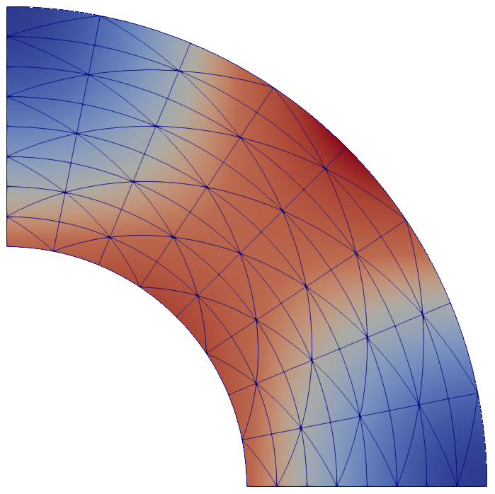
Isoparametric elements:

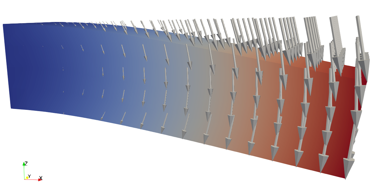
3D problems:

ODE formulation

The DG method leads to the linear system of equations

$A\bm{u} = \bm{b}(\bm{S}, t).$

The on-fault slip and time only affect the right-hand side $\bm{b}$ of the linear system of equations. The operator $A$ stays constant throughout the whole earthquake cycle. On-fault tractions depend linearly on the displacement $\bm{u}$ via a coupling matrix $C$, therefore one can abstractly write

$[\sigma_n(\bm{S}, t), \tau(\bm{S}, t)] = CA^{-1}\bm{b}(\bm{S}, t)$

Hence, the friction relations become

$\begin{aligned} -\tau_i(\bm{S},t) &= \sigma_n(\bm{S},t)f(|V|,\psi) V_i / |V| + \eta V_i \\ \frac{dS_i}{dt} &= V_i\\ \frac{d\psi}{dt} &= g(|V|,\psi)\\ \end{aligned}$

For the algebraic equation the conditions for applying the implicit function theorem are satisfied for many friction laws. Therefore, the slip-rate is a function of slip, state, and time, and we obtain the system of ODEs

$\begin{aligned} \frac{dS_i}{dt} &= V_i(\bm{S}, t, \psi)\\ \frac{d\psi}{dt} &= g(|V(\bm{S}, t, \psi)|,\psi)\\ \end{aligned}$

The evaluation of the right-hand side of above system of ODEs proceeds as follows

1. Set slip boundary condition and solve linear elasticity problem.
2. Solve non-linear friction relation for slip-rate (locally for each on-fault node).
3. Evaluate right-hand side of the system of ODEs with computed slip-rates.

Given that we may evaluate the right-hand side, we can apply any explicit time-stepping to the system of ODEs. We use the TS module from PETSc (Abhyankar et al., 2018), in particular the adaptive Runge-Kutta schemes 3bs, 5dp, or 8vr.

References

1. Rivière, B. (2008). Discontinuous Galerkin Methods for Solving Elliptic and Parabolic Equations. Society for Industrial and Applied Mathematics. https://doi.org/10.1137/1.9780898717440
2. Arnold, D. N., Brezzi, F., Cockburn, B., & Marini, L. D. (2002). Unified Analysis of Discontinuous Galerkin Methods for Elliptic Problems. SIAM Journal on Numerical Analysis, 39(5), 1749–1779. https://doi.org/10.1137/S0036142901384162
3. Abhyankar, S., Brown, J., Constantinescu, E. M., Ghosh, D., Smith, B. F., & Zhang, H. (2018). PETSc/TS: A Modern Scalable ODE/DAE Solver Library. ArXiv Preprint ArXiv:1806.01437.